COVID Modelling: Part 1
As lockdown in Melbourne has been extended, a lot of focus has been placed on the model developed by researchers at the University of Melbourne. People who believe in the modelling say that it is based on significant data, that it is complex and can be fine-tuned to explore a range of different policy scenarios, and that it has been reviewed by specialists in the field. People opposed to the modelling say that it is not based on Victoria-specific data, that it assumed that people “move about on a chessboard”, and that it gives different results based on random chance.
So who is right?
Well, in some ways, both are. And, luckily, the models have been made available for us to play around with, so that we can get them running, see how they work, and try and get some idea of the variability inherent in these kinds of models.
The purpose of this series of posts is to walk you through the University of Melbourne COVID Modelling, from accesing the models, running them on your computer, understanding and adjusting the parameters, and generating and analysing the outputs.
Now, to start with, we will need to get a copy of the models themselves. You can access them on GitHub, by clicking on the green “Code” button and selecting “Download ZIP”. Unzip the file that downloads somewhere on your computer. (Of course, if you are familiar with Git, feel free to clone the repository directly, or to make your own fork of the repository and clone that – all that matters is that you have access to the files.)
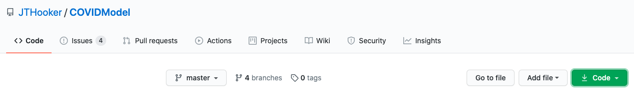
The top bar of the COVIDModel GitHub page
Now, before we go poking around in the model code themselves, it will be helpful to have something that can actually run them. The models are written in NetLogo, a variant of the Logo programming language maintained by Northwestern University. While the webpage for NetLogo may look childish, and indeed it is often used as a teaching tool (with its own souped-up version of the “turtle” that was such a feature of the original Logo experience), it is a powerful and academically rigorous environment for building up simulations of natural phenomena.
Navigate to the NetLogo Downloads page, either by clicking on the link or following the Download link in the top left (note that you do not need to fill in your details to proceed to the Download page), and download the relevant version of NetLogo for your system. I’m working on a MacBook Pro, so I selected the Mac OS X version and downloaded the .dmg file. Once that downloaded to my system and I mounted the disk image, I dragged the entire NetLogo 6.1.1 folder to my /Applications folder to install it. If you’re working on Windows, the download will be a .msi installer, so run that and follow the prompts.
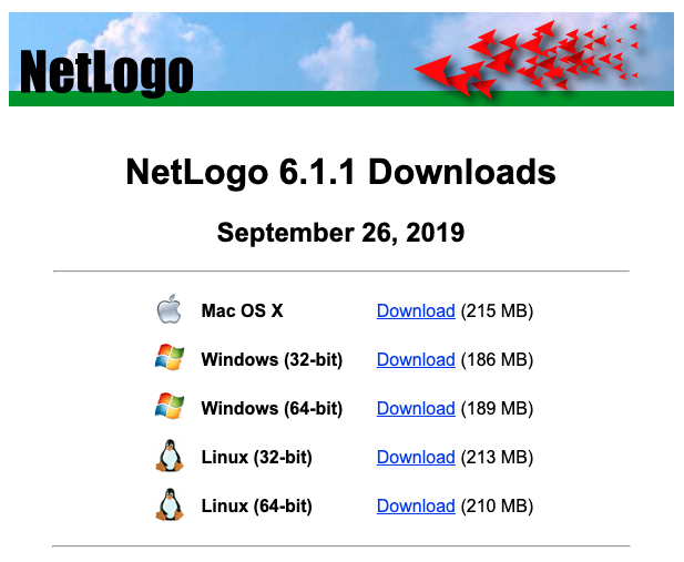
A screenshot of the NetLogo Downloads page
So, now we have the software, let’s take a look at the files that we downloaded!
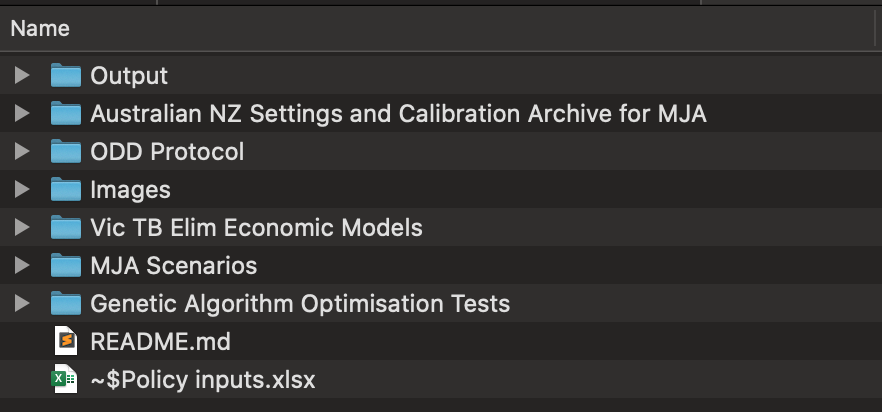
The files in the unzipped folder downloaded from GitHub
In the folder that you unzipped onto your computer, you should have 7 sub-folders, a README file, and an excel spreadsheet. The two files we can essentially ignore - they contain some informational text and an extract of data that is relatively outdated. Let’s take a look at the folders!
- ODD Protocol: The single (to date) file in this folder is an Appendix that describes the models using “the Overview, Design concepts and Details (ODD) protocol for describing Individual and Agent-Based Models (ABMs)”. Reading through this document will give you a deep understanding of the structure and function of the various models, and I have largely based these posts on it. It is, however, rather complex reading, hence these posts!
- Output: This folder contains outputs from existing runs of several of the models. We will be able to re-create versions of these files once we get the models running locally.
- Images: This folder contains images that can be used to show off the model interface, including one that is necessary for some of the code to run!
- Genetic Algorithm Optimisation Tests: This folder contains configuration files for BehaviorSearch 6.1.1, which is bundled with NetLogo. This application allows us to run a model multiple times with different parameters, looking for those parameters that maximise a particular function. As there are often lots of parameters and lots of different values for those parameters, we can’t possibly test them all, so a genetic algorithm is used to try and find optimal values. If you take a look at the file
Test.searchConfig.json, you can see that this particular genetic algorithm was used to find the optimal time to switch between different stages of lockdown in order to minimise the number of active infections, the total number of infections, and the financial cost of the outbreak. - Vic TB Elim Economic Models: The model described here seems to be still under development at the time of writing. It contains some rather complex financial resource modelling as well as the infection and public health data. However, as a public health person and not an economist, I don’t know that I would be able to interpret the output as effectively as I would like - so I’m going to focus on the others.
- Australian NZ Settings and Calibration Archive for MJA: This folder contains calibration data that is used to make the models better fit different scenarios. In particular, these models were originally developed using the earliest available data - from Wuhan Province, China - and have since been adapted to Australia and New Zealand. It also contains one of the models that we’re actually going to be trying out! The model in here is the country-wide model.
- MJA Scenarios: And in here is the model that everyone’s talking about - the Dynamic Policy Model, which models a variety of different policy approaches including physical distancing, mask usage, and usage of the Australian Government’s COVIDSafe mobile app (or similar). The PDF file in this folder,
Vic Simulation Appendix A V1.pdf, details the values that are used in calibrating this model. (Note that this PDF has an incorrect link in the caption for Table 1 - you can find the file that they reference in the ODD Protocol folder.)
Okay, so first up, let’s open up the Victorian model. (I know that you want to see that one!) Next post, we’ll take a step back to the simpler Australia-wide model to get to grips with some of the concepts that underlie models like this - but let’s at least run a model and see what happens, shall we? To do that, double-click on the file COVID SIMULS VIC.nlogo in the MJA Scenarios folder. It should load up in NetLogo, and you should see a screen something like this:
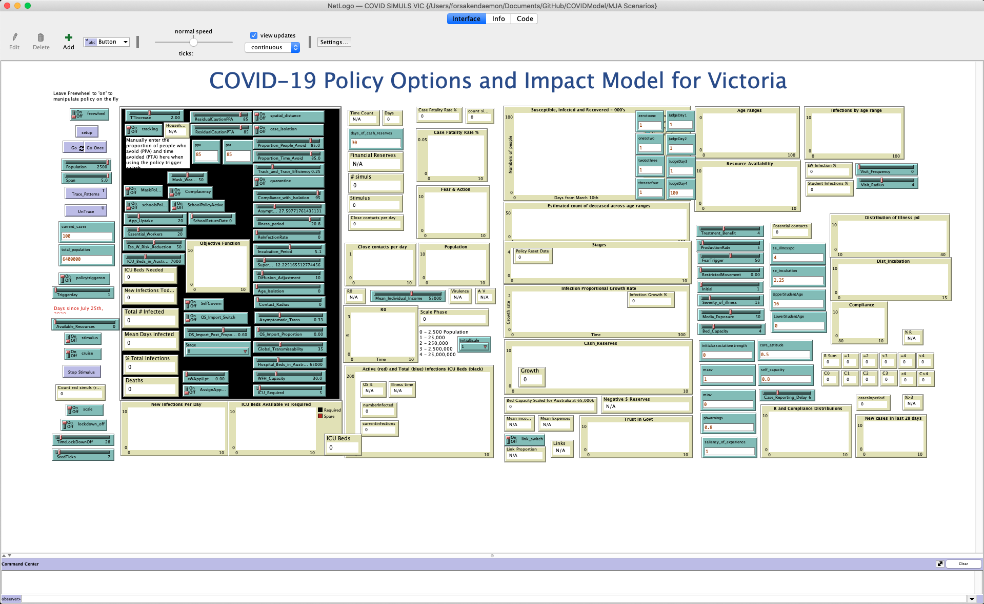
The interface panel for the Victorian COVID model in NetLogo
If you don’t see all of the interface on your screen, you can change the zoom in the Zoom menu.
Towards the top left of the screen, you should see a purplish button labeled “setup”. In NetLogo, to start a simulation from a model we have to create the “agents”, or the people in the simulation. Of course, agents don’t have to be people - they could be animals, cars, or anything else that moves around an environment. Click the setup button.
If you see an error like the following when you click the setup button, the code needs to be updated.
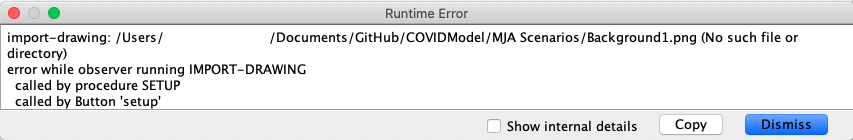
Error when calling setup in certain models
Close the error box, and navigate to the “Code” pane using the buttons at the top of the screen. search for to setup, and in the definition of that procedure, change the line
import-drawing "Background1.png" ;; imports MSD image
to
import-drawing "../Images/Background1.png" ;; imports MSD image
like so: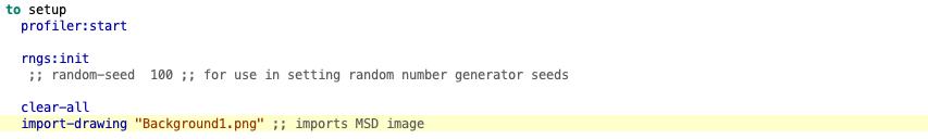
Before making change to the code
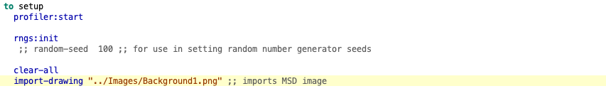
After making change to the code
Navigate back to the “Interface” pane, and click the setup button again.
When you click the setup button, you should see (mostly hidden by lots of sliders and data readouts) lots of blue and red dots appear in the black rectangle on the left. You should also, towards the middle of the screen, see the number “6400000” appear in the “# simuls” box. This refers to the number of people being simulated - 6.4 million.
As a final piece of setup, click on the dropdown towards the top of the screen, under the “view updates” checkbox, that reads “continuous”. Select “on ticks” instead - this will update your view whenever time advances in the simulation, rather than every time something happens in the background - not changing this can make your simulations take an awfully long time to run!
Finally, click the “Go” button towards the left of the screen, with two small arrows in the bottom right-hand corner. Things should start happening! You should see graphs begin to update, the dots in the black rectangle move around busily, and numbers begin to change. Keep an eye on the “Active (red) and Total (blue) infections ICU Beds (Black)” graph towards the bottom, as well as the numeric displays on top of it. Once the number of “currentinfections” reaches zero, click the Go button again to stop the simulation.
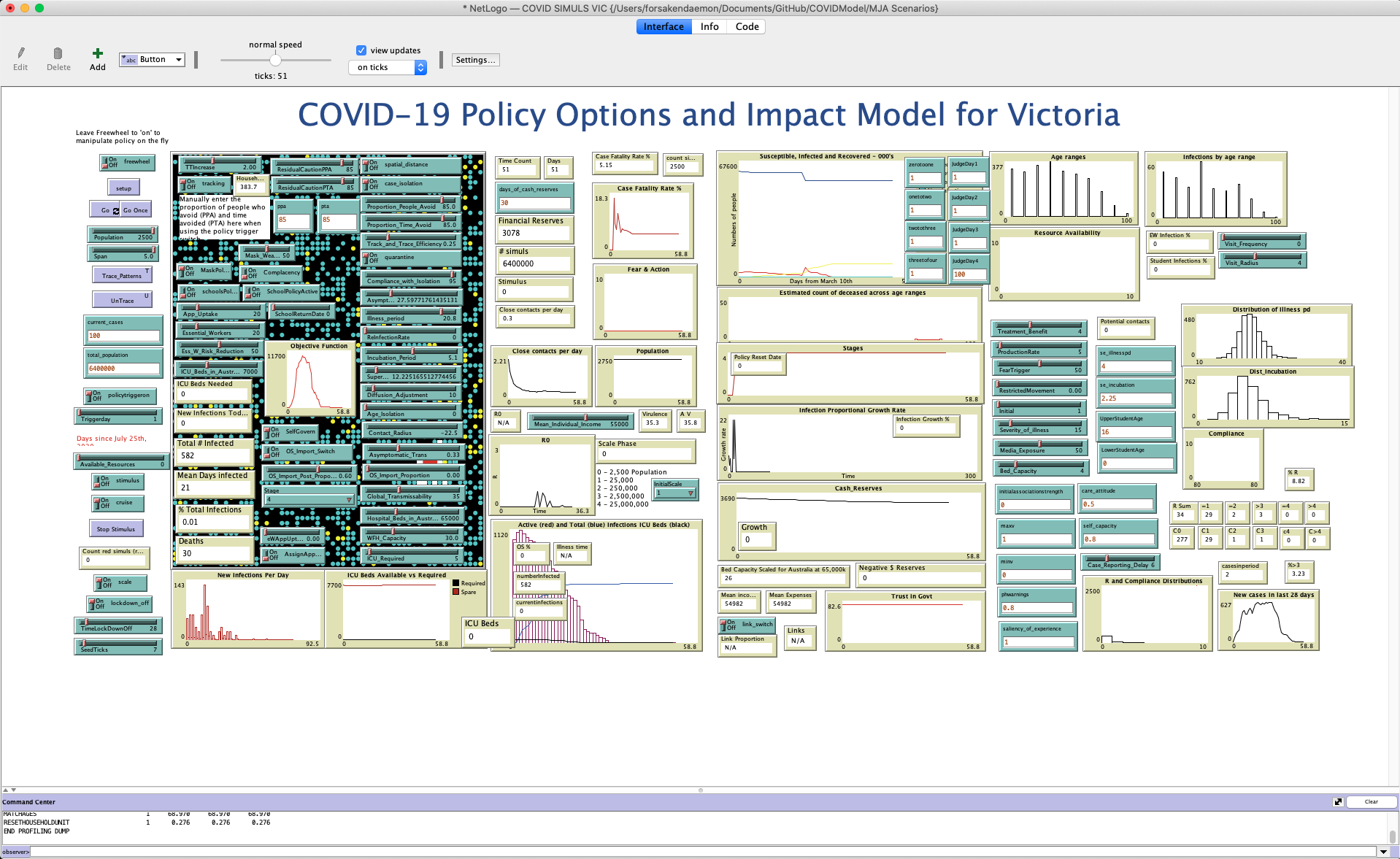
Example interface after running the Victorian COVID model
And there you have it! We just ran a simulation. Every time we run this, it will go slightly differently - the placement of the people, their movements, whether a particular encounter with a person with active infection will result in transmission, and many other aspects of the simulation are all determined randomly, based on what we know about those variables from scientific studies.
In this particular simulation, the state very rapidly went to Stage 4 lockdown - and remained that way to the end of the simulation (see the “Stage” dropdown towards the bottom of the black rectangle, and the “Stages” graph partially hidden by the “Policy Reset Date” readout in the middle of the screen). In this simulation, the policies instituted resulted in elimination of the virus reasonably quickly - no more people have the virus after less than 60 days, although 582 people were infected, and 30 people passed away. The virtual state never ran out of ICU beds, which is a very good sign.
In the next post, we will look into the theory of these kinds of models, and adjust some of the parameters of the Australia-wide model to start to understand what effect different virus features, social policies, and random chance have on the results of these kinds of simulations.