COVID Modelling: Part 2
Well, now that we have the models downloaded and the software installed (if you don’t, check out part 1), it’s time to explore the models that we have. How do they work? What kind of assumptions are they based on?
Note: if you haven’t read it already, you may be interested in the article that the authors of this model wrote for Pursuit at the University of Melbourne, Modelling Victoria’s Escape from COVID-19, which talks about what these models were designed to do and not do in a really nice way.
For this part, we’re going to look at the Australia-wide model that’s in the Australian NZ Settings and Calibration Archive for MJA folder. While it works in much the same way, it’s simpler, which will make it easier to explore its structure! Start off by opening up that folder and then opening COVID SIMULS.nlogo up in NetLogo. As before, while this is a simpler model, there’s still a lot to fit on the screen, so you may need to make the display smaller using the “Zoom” menu.
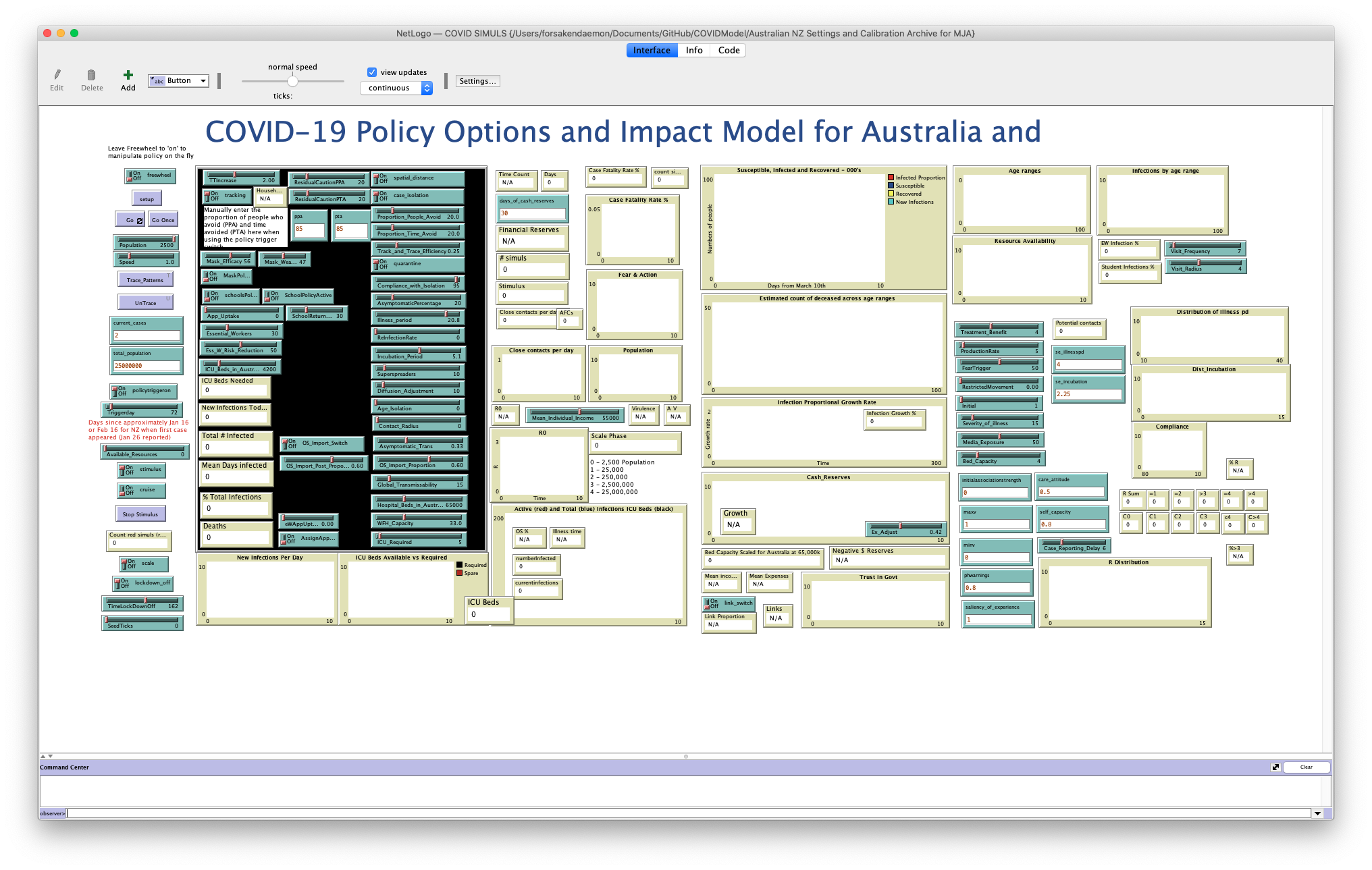
The (suitably zoomed-out) Interface view for the model that we will be exploring.
Again, we can set up the simulation by clicking on the “setup” button, and run a simulation by clicking on “Go” just below it. If you find that it runs slowly, make sure that “view updates” are set to only happen “on ticks” at the top of the screen, so that the view only updates when time ticks forward, rather than every time that something happens in the simulation. Watch the simulation until the number of “currentinfections” towards the bottom of the screen (overlapping the “Active (red) and Total (blue) Infections ICU Beds (black)” graph) reaches zero.
Note that various different things can happen: in the simulation below, there was an initial spike in infections, followed by a long and slow recovery period with a small second wave. In this case, roughly 4.37% of the simulated population were infected (a total of 10,928 people) for an average of 21 days each, and 113 people died.1
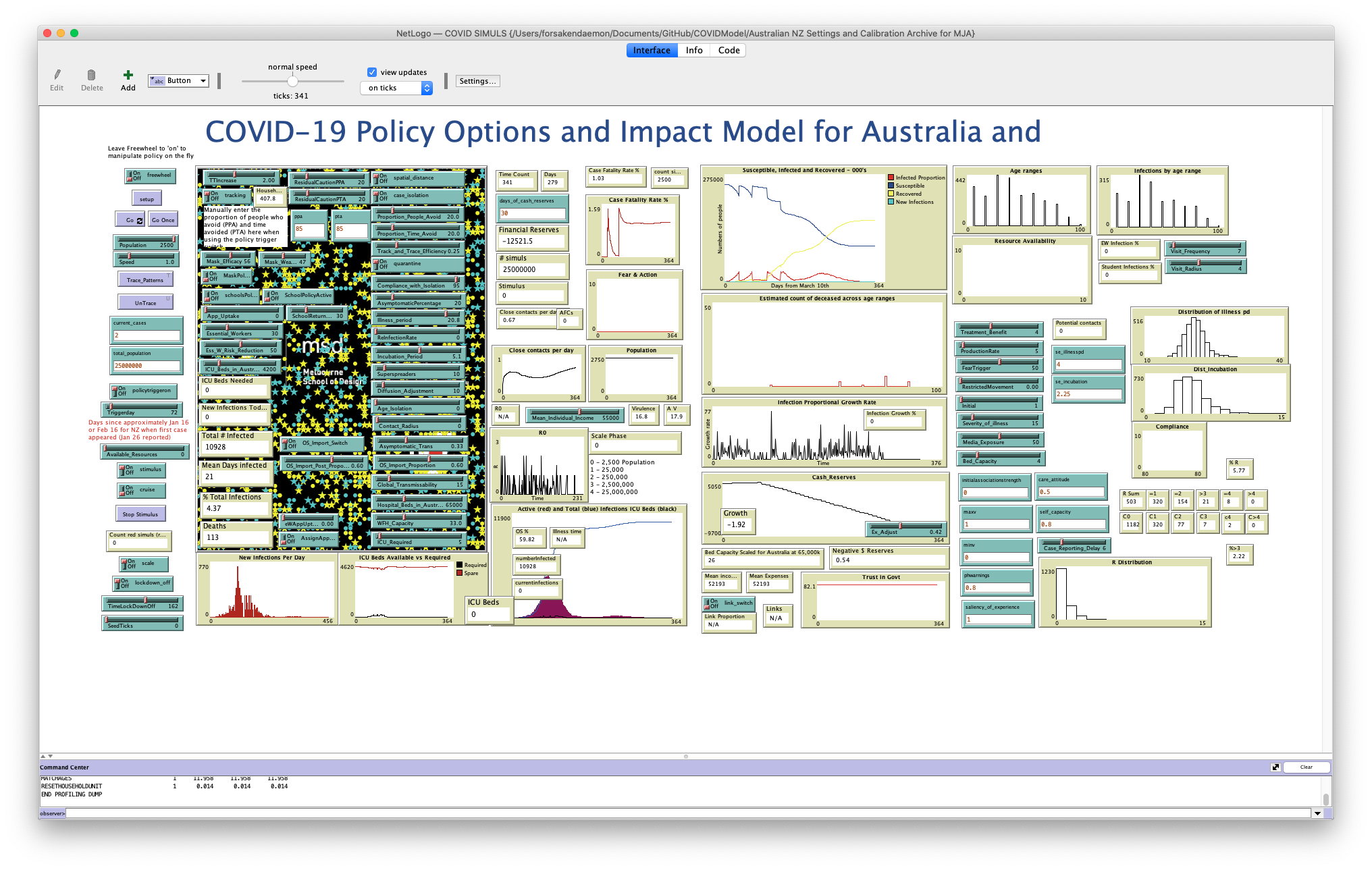
Results of a running model.
So what’s actually going on under the hood here? Well, to understand that, let’s head over the the “Code” tab.
If you click on the Code tab, the first thing that you’ll see will be the extensions that are loaded. For this model, there’s the rngs extension, which allows for the (predictable) generation of pseudorandom numbers, and the profiler extension that provides profiling functions that measure the time that particular operations take. Luckily, both of these extensions come bundled with NetLogo – which we can check using the “Extensions Manager”, which you should be able to access using the “Tools” Menu. Look for entries named “Expanded Random Number Generator” and “Profiler” respectively.
After the extensions sectio, there’s a large globals section. This section of the code contains all of the global variables – variables that can be accessed and modified by any of the code, rather than only being available in particular sections of the code. While for the Victoria-specific model many of these variables are defined in the ODD Protocol, starting on about page 6, we don’t have a protocol document like that for this model, so we have to infer the meaning of many of them. However, the names are helpful here: numberInfected is the number of people who have been infected with the disease since the beginning of the simulation, CaseFatalityRate is an estimate of the Case Fatality Rate (the number of people who have been diagnosed with a disease who have died), and DeathCount is a count of the number of people who have died of the disease so far in the simulation. Helpfully, we have seen several of these before, displayed on the Interface view: the numberInfected is displayed both as the “Total # Infected” towards the left of the screen, and as the “numberInfected” that we watched before, for example.
After the globals section we see the breed section. The word “breed” here is a noun, meaning a particular kind of animal, not a verb. NetLogo uses breed to mean a kind of agent (referred to in NetLogo as a “turtle”) that it is able to simulate, with different breeds behaving in different ways (although all agents of a particular breed behaving according to the same rules). This model defined four different kinds of agents: “simuls”, “resources”, “medresources”, and “packages”. The breed keyword defines how we will refer to all of the agents of the breed at once (“simuls”, for example) and how we will refer to just one of them at a time (“simul”). The breed command then creates some helper keywords that make creating, identifying, and finding agents of a particular breed easier. For most of the rest of this post, we are going to focus largely on simuls, as they’re the most complex agents in the model.
We then use the directed-link-breed keyword to create a type of link. A link is just a line between two of the agents that we defined before. Here, the link is directed - it’s an arrow pointing from one agent to another. Similarly to the previous section, this model will call the collection of all of these links red-links, and only one of them a red-link.
Now, we get to see one of those special keywords that the bred keyword created for us! simuls-own is similar to the globals keyword that we saw before, in that it creates variables. Instead of there only being one copy of each of these variables, though, there’s one of each “wrapped up” inside any simuls that we might create. By looking down this list of variables, we can see what simuls represent: each one represents a person in our simulation, who may or may not have the disease (whether someone is currently infected is determined by the color of the simul, which is built into NetLogo, and so doesn’t need a separate variable). Each simul has a range of characteristics, such as:
- their baseline
health, - the
Pacewith which they can move around (since some people will not move around very much, and therefore are less likely to come into contact with new people), - whether they are an Essential Worker or a Student (defined by their
EssentialWorkerFlagandStudentFlag), - the amount of
PersonalTrustthat they have in Government, - how old they are, grouped into an
AgeRange, and - both their concern about protecting themselves and others from infection (
CareAttitude) and their capacity to feel that concern (SelfCapacity).
Importantly, these variables can change over the course of a simulation (although some, like their AgeRange, are assumed to stay reasonably constant). By then looking at how these variables change, we can get an understanding of how, for example, overall trust in Government is likely to change, and what effect that may have on a population’s likelihood of complying with Governmental directives, and therefore on the spread of a disease.
Below the set of variables assigned to simuls, you can also see the variables contained within packages, resources, and medresources. You will also see a section labelled patches-own, which details values that are assigned to patches: places in the virtual world in which our agents will be moving around. Patches work somewhat like agents in that they can have variables that are different from patch to patch, although they cannot move around and are generally referred to by x- and y-coordinates.
The effect of each of these variables on a particular agent’s behaviour is modelled using functions, which we will get to in the next post. You can check on the particular value of a variable (for example, health) for a random simul by going to the Interface tab, going down to the Command Center at the bottom, and typing in:
show [health] of one-of simuls
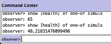
Results of asking NetLogo for the health of one of the simuls.
In this case, I typed this in twice, and each time NetLogo chose a random simul and told me the value of their health: 65 for the first, and 48.21831476099496 for the second.
This idea may cause you some concern: what does it mean to have a particular level of “health” or “trust in Government”? And how do we know what a particular value actually means in terms of an agent’s behaviour? Well, the simple answer is that we don’t: the values that a particular agent has (or can have) are somewhat arbitrary, and often scaled to be within a range from 0–1 or 0–100. What we do know, however, is how people, on average, tend to behave, and we can use that information to set these values to something that makes sense for our model. We then use random numbers to make predictions about what people may or may not do.
For a worked example of how this works, click here!
For example, let’s say that we want to simulate whether people brush their teeth in the morning. We know that:
- about two in every six people brush their teeth “only occasionally”, about a quarter of mornings;
- about one in six people brush their teeth “every day”, and
- the remainder brush their teeth “about half” of mornings.
Well, we can create a variable for each person, brushTeeth, that shows how likely that particular person is to brush their teeth each day on average. There’s a 2-in-6 chance that they’re an “only occasionally” person with a probability of 0.25 on average, a 1-in-6 chance that they’re an “every day” kind of person with a probability of 1.0, and an 3-in-six chance that they’re an “about half” kind of person with a probability of 0.5. So, when we create our simulated sample of people, we roll a standard six-sided die for each person: if the result is a 1 or a 2, then we set their brushTeeth value to 0.25; if it’s a 3, 4, or 5 then we set it to 0.5; and if it’s a 6 then we set it to 1.0.
Because I’m a nerd, and will welcome any excuse to play with dice, I simulated twelve people, and got the results below! You can see that seven of the twelve are “about half” people (a little more than the six we expect), three are “only occasionally” people (a little fewer than the four we might expect), and the remaining two are “every day” people.
| Person | Die value | Type of teeth brusher | brushTeeth |
|---|---|---|---|
| A | 5 | About half | 0.5 |
| B | 1 | Only occasionally | 0.25 |
| C | 5 | About half | 0.5 |
| D | 4 | About half | 0.5 |
| E | 6 | Every day | 1.0 |
| F | 2 | Only occasionally | 0.25 |
| G | 1 | Only occasionally | 0.25 |
| H | 5 | About half | 0.5 |
| I | 5 | About half | 0.5 |
| J | 5 | About half | 0.5 |
| K | 6 | Every day | 0.25 |
| L | 4 | About half | 0.5 |
Now, let’s say that we want to simulate whether people brushed their teeth on a particular day. Well, for each person we now generate a random number from 0 to 1, and look at whether it is greater or less than the value of brushTeeth that we set for that person. If it is less than or equal to their brushTeeth value, then we will say that they did brush their teeth; if greater than their brushTeeth value, then they didn’t. After generating some random numbers (using centile die), I updated the table. It seems that only 6 people brushed their teeth today! There seems to be some opportunity to encourage teeth-brushing in our simulated sample.
| Person | Die value | Type of teeth brusher | brushTeeth | Random | Brushed teeth? |
|---|---|---|---|---|---|
| A | 5 | About half | 0.5 | 0.63 | No |
| B | 1 | Only occasionally | 0.25 | 0.04 | Yes |
| C | 5 | About half | 0.5 | 0.82 | No |
| D | 4 | About half | 0.5 | 0.05 | Yes |
| E | 6 | Every day | 1.0 | 0.11 | Yes |
| F | 2 | Only occasionally | 0.25 | 0.95 | No |
| G | 1 | Only occasionally | 0.25 | 0.98 | No |
| H | 5 | About half | 0.5 | 0.24 | Yes |
| I | 5 | About half | 0.5 | 0.38 | Yes |
| J | 5 | About half | 0.5 | 0.73 | No |
| K | 6 | Every day | 1.0 | 0.64 | Yes |
| L | 4 | About half | 0.5 | 0.56 | No |
The important thing about modelling people like this is that we can make the simulations match, arbitrarily closely, what we have from real-world data. By tweaking the probabilities of a particular variable within an agent, we can make our model match very closely what we see in the long run in the real world. Even better, by gathering data about how people change their behaviour over time, we can develop ways of changing the variable for each agent so that our model matches the real world as well – and this process will work for anything that we might be able to observe in a population. This ability to update the values that the model is using based on observable information is very powerful, as it allows us to run simulations of a model based on what we know about “people in general”, and then to fine-tune the model as data about a particular population become available.
This is partly the basis of he criticism that the Victorian modelling isn’t based on entirely current or Victoria-specific data. When designing a mode in the first place, we need to use estimates of data from a range of different studies conducted around the world. For example, data on the infectivity and lethality of the virus has been estimated by combining case numbers and experiences from earlier outbreaks (particularly for COVID, the earliest outbreaks in Wuhan, China). In addition, the understandings of how people move around Melbourne and Victoria were originally developed as part of urban planning research, not repurposed for a very different purpose! Without using “good enough” data until updated understandings become available, this kind of modelling cannot give predictions. However, the quality of the input data is always important, and so ensuring that models like these are updated as more data become available.
So now we know what all of the pieces of our model are! However, we haven’t actually created any agents yet – and they certainly haven’t started interacting with each other. In the next post, we will setup a simulation, and understand what happens when we run it.
Note that if you try and work out what the actual population and numbers are, you will find yourself off by one or more orders of magnitude. The model will rescale itself depending on how many people are infected to ensure that simulations can actually run on a reular computer, as simulating 25,000,000 individuals at once is challenging for even powerful machines, which is likely what is going on here. ↩︎